Run eDITH with BayesianTools based on joint eDNA and direct sampling data
run_eDITH_BT_joint.RdFunction that runs a Bayesian sampler estimating parameters of an eDITH model fitted on both eDNA and direct sampling data.
Usage
run_eDITH_BT_joint(data, river, covariates = NULL, Z.normalize = TRUE,
           use.AEM = FALSE, n.AEM = NULL, par.AEM = NULL,
           no.det = FALSE, ll.type = "norm", source.area = "AG",
           mcmc.settings = NULL, likelihood = NULL, prior = NULL,
       sampler.type = "DREAMzs",
           tau.prior = list(spec="lnorm",a=0,b=Inf, meanlog=log(5),
                        sd=sqrt(log(5)-log(4))),
           log_p0.prior = list(spec="unif",min=-20, max=0),
           beta.prior = list(spec="norm",sd=1),
           sigma.prior = list(spec="unif",min=0,
                        max=max(data$values[data$type=="e"],
                na.rm = TRUE)),
           omega.prior = list(spec="unif",min=1,
                        max=10*max(data$values[data$type=="e"],
                na.rm = TRUE)),
           Cstar.prior = list(spec="unif",min=0,
                        max=max(data$values[data$type=="e"],
                na.rm = TRUE)),
           omega_d.prior = list(spec="unif",min=1,
                                max=10*max(c(0.11, data$values[data$type=="d"]),
                na.rm = TRUE)),
           alpha.prior = list(spec="unif", min=0, max=1e6),
           verbose = FALSE)
Arguments
- data
eDNA and direct observation data. Data frame containing columns
ID(index of the AG node/reach where the sample was taken),values(value of the eDNA or direct measurement) andtype(equal to"e"for eDNA data and to"d"for direct observation data). eDNA values are expressed as concentration or number of reads; direct observations are expressed as numbers of individuals.- river
A
riverobject generated viaaggregate_river.- covariates
Data frame containing covariate values for all
riverreaches. IfNULL(default option), production rates are estimated via AEMs.- Z.normalize
Logical. Should covariates be Z-normalized?
- use.AEM
Logical. Should eigenvectors based on AEMs be used as covariates? If
covariates = NULL, it is set toTRUE. IfTRUEandcovariatesare provided, AEM eigenvectors are appended to thecovariatesdata frame.- n.AEM
Number of AEM eigenvectors (sorted by the decreasing respective eigenvalue) to be used as covariates. If
par.AEM$moranI = TRUE, this parameter is not used. Instead, the eigenvectors with significantly positive spatial autocorrelation are used as AEM covariates.- par.AEM
List of additional parameters that are passed to
river_to_AEMfor calculation of AEMs. In particular,par.AEM$moranI = TRUEimposes the use of AEM covariates with significantly positive spatial autocorrelation based on Moran's I statistic.- no.det
Logical. Should a probability of non-detection be included in the model?
- ll.type
Character. String defining the error distribution used in the log-likelihood formulation. Allowed values are
norm(for normal distribution),lnorm(for lognormal distribution),nbinom(for negative binomial distribution) andgeom(for geometric distribution). The two latter choices are suited when eDNA data are expressed as read numbers, whilenormandlnormare better suited to eDNA concentrations.- source.area
Defines the extent of the source area of a node. Possible values are
"AG"(if the source area is the reach surface, i.e. length*width),"SC"(if the source area is the subcatchment area), or, alternatively, a vector with lengthriver$AG$nodes.- mcmc.settings
List. It is passed as argument
settingsinrunMCMC. Default islist(iterations = 2.7e6, burnin=1.8e6, message = TRUE, thin = 10).- likelihood
Likelihood function to be passed as
likelihoodargument tocreateBayesianSetup. If not specified, it is generated based on argumentsno.detandll.type. If a custom likelihood is specified, a custompriormust also be specified.- prior
Prior function to be passed as
priorargument tocreateBayesianSetup. If not specified, it is generated based on the*.priorarguments provided. If a user-defined prior is provided, parameter names must be included inprior$lower,prior$upper(see example).- sampler.type
Character. It is passed as argument
samplerinrunMCMC.- tau.prior
List that defines the prior distribution for the decay time parameter
tau. See details.- log_p0.prior
List that defines the prior distribution for the logarithm (in base 10) of the baseline production rate
p0. See details. Ifcovariates = NULL, this defines the prior distribution for the logarithm (in base 10) of production rates for allriverreaches.- beta.prior
List that defines the prior distribution for the covariate effects
beta. See details. If a singlespecis provided, the same prior distribution is specified for allbetaparameters. Alternatively, ifspec(and the other arguments, if provided) is a vector with length equal to the number of covariates included, different prior distributions can be specified for the differentbetaparameters.- sigma.prior
List that defines the prior distribution for the standard deviation of the measurement error when
ll.typeis"norm"or"lnorm". It is not used ifll.type = "nbinom". See details.- omega.prior
List that defines the prior distribution for the overdispersion parameter
omegaof the measurement error whenll.type = "nbinom". It is not used ifll.typeis"norm"or"lnorm". See details.- Cstar.prior
List that defines the prior distribution for the
Cstarparameter controlling the probability of no detection. It is only used ifno.det = TRUE. See details.- omega_d.prior
Prior distribution for the overdispersion parameter for direct sampling density observations.
- alpha.prior
Prior distribution for the inverse DNA shedding rate (i.e., the organismal density that sheds a unit eDNA value per unit time).
- verbose
Logical. Should console output be displayed?
Details
The arguments of the type *.prior consist in the lists of arguments required by dtrunc
(except the first argument x).
By default, AEMs are computed without attributing weights to the edges of the river network.
Use e.g. par.AEM = list(weight = "gravity") to attribute weights.
Value
A list with objects:
- param_map
Vector of named parameters corresponding to the maximum a posteriori estimate. It is the output of the call to
MAP.- p_map
Vector of best-fit eDNA production rates corresponding to the maximum a posteriori parameter estimate
param_map. It has length equal toriver$AG$nNodes.- C_map
Vector of best-fit eDNA values (in the same unit as
data$values, i.e. concentrations or read numbers) corresponding to the maximum a posteriori parameter estimateparam_map. It has length equal toriver$AG$nNodes.- probDet_map
Vector of best-fit detection probabilities corresponding to the maximum a posteriori parameter estimate
param_map. It has length equal toriver$AG$nNodes. If a customlikelihoodis provided, this is a vector of null length (in which case the user should calculate the probability of detection independently, based on the chosen likelihood).- cI
Output of the call to
getCredibleIntervals.- gD
Output of the call to
gelmanDiagnostics.- covariates
Data frame containing input covariate values (possibly Z-normalized).
- source.area
Vector of source area values.
- outMCMC
Object of class
mcmcSamplerreturned by the call torunMCMC.
Moreover, arguments ll.type (possibly changed to "custom" if a custom likelihood is specified), no.det
and data are added to the list.
Examples
data(wigger)
data(dataCD)
# reduce number of iterations for illustrative purposes
# (use default mcmc.settings to ensure convergence)
settings.short <- list(iterations = 1e3, thin = 10)
set.seed(1)
out <- run_eDITH_BT_joint(dataCD, wigger, mcmc.settings = settings.short)
#> Covariates not specified. Production rates will be estimated
#> based on the first n.AEM = 26 AEMs.
#>
Running DREAM-MCMC, chain 1 iteration 300 of 1002 . Current logp 1556.836 1482.211 1585.538 Please wait!
Running DREAM-MCMC, chain 1 iteration 600 of 1002 . Current logp 1557.273 1527.394 1585.538 Please wait!
Running DREAM-MCMC, chain 1 iteration 900 of 1002 . Current logp 1559.214 1529.97 1604.182 Please wait!
Running DREAM-MCMC, chain 1 iteration 1002 of 1002 . Current logp 1559.214 1529.97 1604.182 Please wait!
#> runMCMC terminated after 2.171seconds
#> gelmanDiagnostics could not be calculated, possibly there is not enoug variance in your MCMC chains. Try running the sampler longer
# \donttest{
library(rivnet)
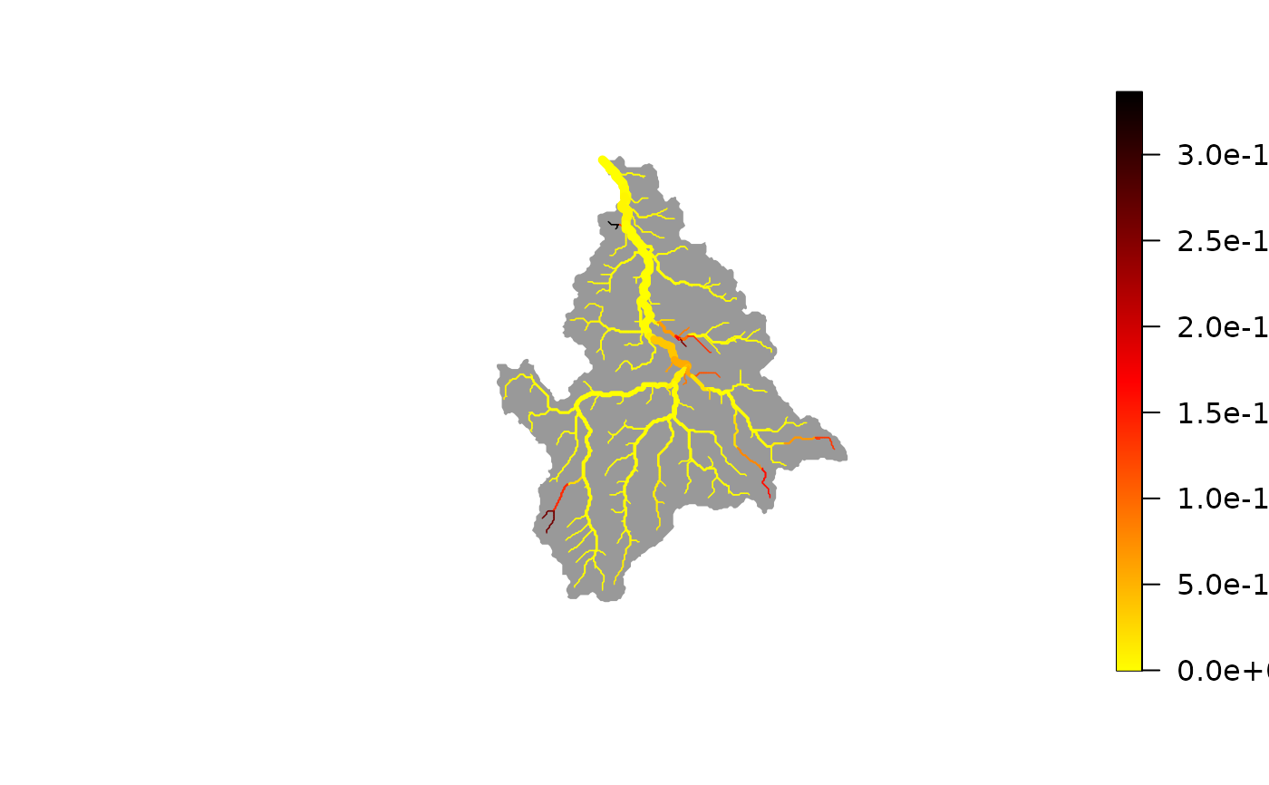
# best-fit (maximum a posteriori) map of eDNA production rates
plot(wigger, out$p_map)
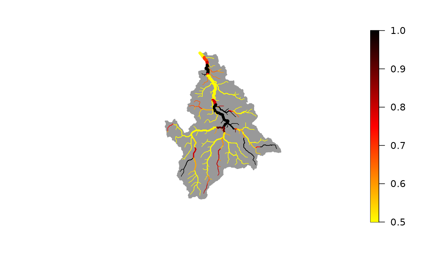
 # best-fit map (maximum a posteriori) of detection probability
plot(wigger, out$probDet_map)
# best-fit map (maximum a posteriori) of detection probability
plot(wigger, out$probDet_map)
 # compare best-fit vs observed values
data.e <- which(dataCD$type=="e")
data.d <- which(dataCD$type=="d")
plot(out$C_map[dataCD$ID[data.e]], dataCD$values[data.e],
xlab="Modelled (MAP) eDNA concentrations", ylab="Observed eDNA concentrations")
abline(a=0, b=1)
# compare best-fit vs observed values
data.e <- which(dataCD$type=="e")
data.d <- which(dataCD$type=="d")
plot(out$C_map[dataCD$ID[data.e]], dataCD$values[data.e],
xlab="Modelled (MAP) eDNA concentrations", ylab="Observed eDNA concentrations")
abline(a=0, b=1)
 plot(out$p_map[dataCD$ID[data.d]], dataCD$values[data.d],
xlab="Modelled (MAP) eDNA production rate", ylab="Observed density data")
plot(out$p_map[dataCD$ID[data.d]], dataCD$values[data.d],
xlab="Modelled (MAP) eDNA production rate", ylab="Observed density data")
 # }
# }